Introduction to Elasticsearch
Elasticsearch (ES) is a distributed open-source search and analytics engine built on the text search library Apache Lucene. Given enough machines, an ES cluster can typically execute search and aggregation queries across very large datasets. While ES is great if you want traditional full text search over a set of text documents (similar to Google search), it is also very useful for searching and aggregating over large sets of more structured or semi-structured datasets like system logs, network traffic data and collected system metrics.
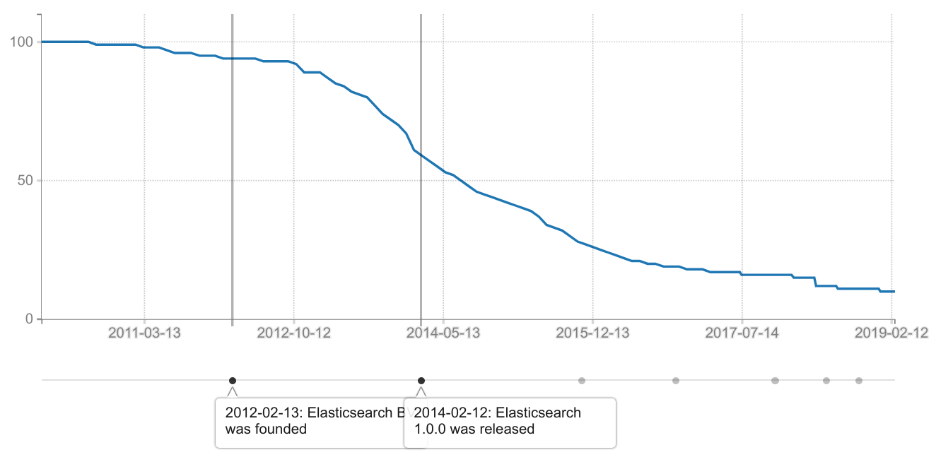
The very first version of Elasticsearch (0.4.0) was written by Shay Banon (kimchy) who is the current CEO of Elastic. The very first version of ES was published on Github Feburary 8th 2010. Shay had previously (2006-2010) developed another search related open source project called Compass1 which was a high level API wrapping Lucene that also added a few features. After 209 days, the first PR by another developer was merged into ES, by that time kimchy had managed to land an incredible 1145 additional commits (5.5 commits per calendar day). Clearly, Shay knew very well both what he wanted to build and how it should be built. On 13th Feb 2012, Shay created the company “Elasticsearch BV” together with Steven Schuurman (who became the initial CEO), Uri Boness and Simon Willnauer.
Steven Schuurman had previous co-founded various other companies. Before Elastic he was the CEO of Orange11, a software company that amongst other things developed enterprise search solutions based on Solr / Lucene. Uri Boness has been working as “Software Architecture / Head of Search” at Orange11 and Simon Willnauer was (and still is) a core committer in the Apache Lucene project.
Two years later, on the 12th Feburary 2014, Elasticsearch 1.0 was released. Shay Banon eventually took over the CEO role in early 2017, even though he was still committing code up to mid-2015. In fact, a quick “git log” in the ES repo reveals that the developer with the most commits is still, to this day, Shaw Banon. Here is a graph showing “how many percent of ES commits to date that was authored by kimchy” :
Meanwhile, Jordan Sissel had been working on Logstash (an open source ruby/java based ingestion tool that could process and stash log data into multiple backends). Logstash predated Elasticsearch but using Logstash with Elasticsearch became very common and Jordan joined Elastic in 20132. Similarly, Kibana was an open source project for visualizing and working with Elasticsearch data. It started outside of Elastic but Rashid Khan, who worked for Elastic, quickly became the lead developer. Because Elastic grew out of various open source projects, it also grew into a very distributed company with employees in over 35 countries and quite a few employees working remote. Elastic NV eventually filed for an IPO in June 2018 and was listed on the New York Stock Exchange in October 2018. The IPO was at $36 per stock but they closed at $70 after the first trading day. The ESTC market cap is 6.11B as of today, and at the time of the IPO, Schuurman owned a 19 percent stake and Banon owned 12 percent.
The Elastic stack
ES is often used together with Logstash and Kibana (forming the ELK-stack). Logstash is a tool for processing data from log files and feeding them into ES (it has plugins for inputs, transforms and outputs so it’s essentially an ETL tool), and Kibana is a web UI that allows you to query ES using search queries in Lucene syntax. Kibana also lets you aggregate data and render it into various charts and visualizations. It is implemented in typescript with a node backend and React for the frontend. The Elastic stack also includes a set of programs, referred to as “Beats”, that feed various other kinds of data into ES (sometimes via Logstash). Examples include FileBeat (feeds file data like logs into ES), MetricBeat (collects system metrics like CPU/network/memory usage and feeds it into ES) and PacketBeat (records network traffic and feeds it into ES).
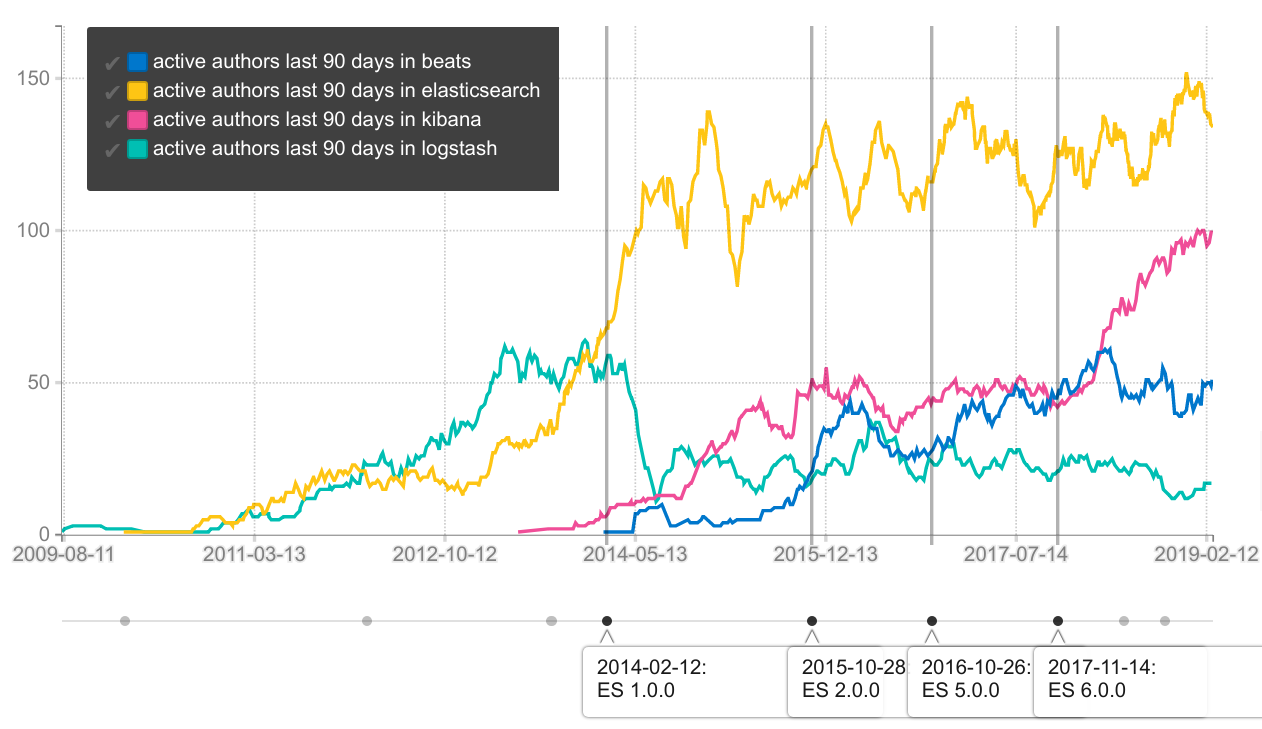
This chart shows the number of unique git authors seen per 90 days for the major Elastic.co repositories:
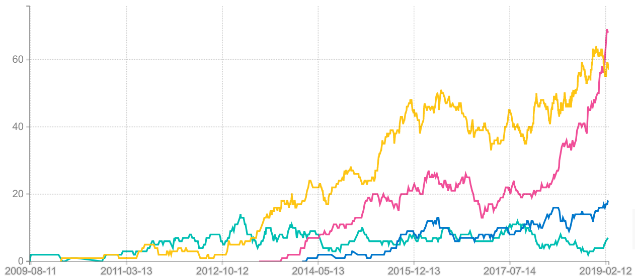
The above chart includes some open source “one-off patching”, and if you instead count the number of unique git authors that had 5 or more commits in each 90 day window, you get this chart instead (I suspect this latter metric is better correlated with the actual number of full time developers working on a project).
Example: How the Elastic stack can work together to process logs
When collecting system logs, a common setup is to run FileBeat on each machine and have it send data to Logstash. Logstash will then parse the raw log files into sets of field values to make them more search friendly (this is referred to as “grokking”). For example, if your log lines have the following format:
2019-02-17 00:05:02,061 INFO FoobarComponent  Connecting to service at foo:1234
2019-02-17 00:05:03,038 DEBUG FoobarComponent  Loaded 60 objects.
2019-02-17 00:05:04,012 DEBUG CoreComponent  Finished initialization.
You can use grokking to indicate that the first two “words” are a timestamp, the third word is a log level, the fourth word is a component name and the rest is the “log message”. You can define custom grokking using regexp patterns etc, or you can rely on pre-defined grok patterns that ships with Logstash (it knows how to parse common log file types like Apache access/error logs etc). Once the data is sent to ES the log lines will have been translated to something like this instead:
{
    "timestamp": "2019-02-17 00:05:02,061",
    "severity": "INFO",
    "component": "FoobarComponent",
    "message": "Connecting to service at foo:1234",
}
In the end, this makes it possible to find this data in Kibana (or
programmatically via ES) using a query like severity:INFO AND
message:connecting.
Before FileBeat existed a lot of people ran Logstash directly on each node but it’s written in Ruby + Java so it typically consumes quite a lot of memory compared to FileBeat (which is implemented using the Go programming language). Also FileBeat is more lightweight because, unlike Logstash, it only forwards data; it doesn’t know how to parse hundreds of different log formats etc. Another nice benefit is that the network protocol used between FileBeat and Logstash has a notion of back-pressure so if the Logstash server gets overloaded it can tell FileBeat to slow down a bit temporarily and spool the data. Searching logs is of course just one use case for ES among many many others.
Why non “full text search” queries are not good enough
Before adding ES to your infrastructure it’s important to understand what
problem it solves and why. Suppose you want to implement full text search over a
SQL database of “products”, where each product has a .title,
.description and set of comments (stored in a different table). It’s not
really possible to implement search using a crude solution like:
...
   FROM products p
   LEFT JOIN comments c ON (p.product_id = c.product_id)
   WHERE
        p.title LIKE '%searchstring%' OR
        p.description LIKE '%searchstring%' OR
        c.comment_text LIKE '%searchstring%'
There are many reasons why the above query won’t work well. The database cannot
build an index for this so this type of query will be slow unless the table is
really small. If the user searches for word1 word2 they will get no
results even if a product contains word2 word1 in the description. If the
user searches for satisfies, documents containing satisfy will not
be returned. Each item will either match the condition or it will not, the
database will not rank the search results. For example, if “productA” has the
search term both in its title and in its description but “productB” only had the
search term in its description, then it would be reasonable to expect that
“productA” would be returned as the top search result but the SQL query won’t
ensure that.
In relational databases you should normalize the data, splitting it into many tables and connecting them with foreign keys (this helps ensure that there is one source of truth and that the data is consistent). However, when you implement a search feature you typically want to search in several of these fields / columns so you are often forced to JOIN the data which can be expensive. If a row points at another row via a foreign key, those rows needs to live on the same machine / shard for the JOIN to be efficient; so the more such dependencies you have within the data, the more difficult it becomes to do horizontal scaling / efficient automatic sharding.
Wait, what about the built-in full text search in my RDBMS ?
If you dip into vendor specific SQL, most RDBMS have some sort of “full text index” that you can create for a text column to mitigate the matching issues above.
For example, PostgreSQL actually offers two different kinds of full text search indices. GIN based full text indexes are very fast for searching but slower to build and take up more space (these are based on an “inverted index” just like ES). GIST based indexes are slower for searching (but still pretty fast) while providing faster inserts / updates. Creating and searching using a PostgreSQL GIN index is quite straightforward:
ALTER TABLE products ADD "product_vectors" tsvector;
CREATE INDEX idx_fts_vec ON products USING gin(product_vectors);
INSERT INTO products
    (id, title, description, product_vectors)
VALUES (
    42,
    'Nikon D5',
    'The Nikon D5 is a full frame professional DSLR camera',
    (
        to_tsvector('Nikon D5') ||
        to_tsvector('The Nikon D5 is a full frame professional DSLR camera') ||
        to_tsvector('wow super nice camera') /* <-- text from comments */
    )
);
/* The actual search is done using: */
SELECT id FROM products WHERE product_vectors @@ to_tsquery('searchword');
Now, if you already depend on the SQL database, then using the built-in full text search saves you having to install, integrate, upgrade and maintain separate software for handling search. Another benefit of using the built-in full text search is that the database can automatically keep the full text index up-to-date, just like it does with a regular database index. With Elasticsearch, the application has to submit a re-indexing request to ES whenever the SQL data changes (so there will typically be a short period of time where the data is out of sync). On the other hand, rebuilding a GIN-index in PostgreSQL for example, can be quite expensive and it really depends on your use case whether you want this to happen immediately or not.
If your dataset is small enough, or if search is not a primary focus for your users; you might might get away with using built-in full text indices. For example, Stackoverflow used3 this approach for the first few years, before they switched to Elasticsearch.
Built-in full text search works until it doesn’t
One of the main arguments against built-in full text indices is that the RDBMS typically is the least scalable part of your infrastructure, so anything that can move a significant fraction of the load elsewhere is valuable. Elasticsearch also offers much better fine-tuning / customization of the full text indexing process. This gives you more detailed control over which search terms should match which documents (e.g. the matching of “satisfy” vs “satisfies” in the above example).
Another key benefit is that even if the data is normalized in the SQL server, you can index it in denormalized form in Elasticsearch. From the example above, above we can create a single “document” in ES that contains the product title, description and all the comments for that product. In practice, this means that with ES you get horizontal scaling that actually works.
In general, you have to think carefully about:
- how much space are you willing to allocate for the index
- how fast must the search queries execute
- how important is horizontal scaling
- how fine-tuned control over indexing / search matching do you need
- how quick must the re-indexing be
Competitors to Elasticsearch
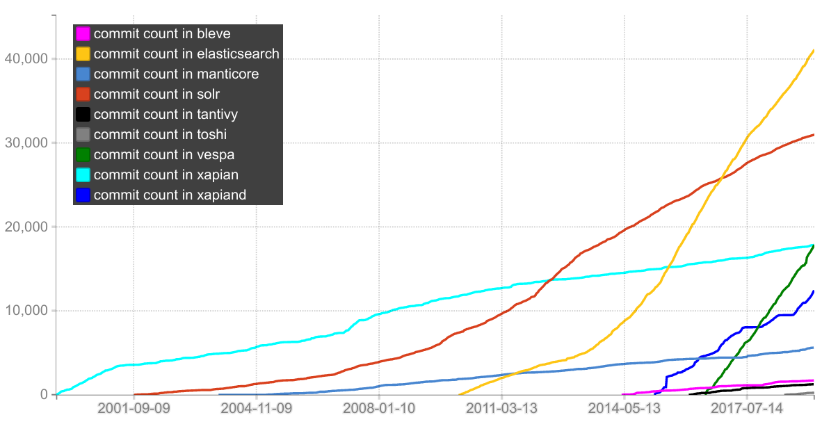
Even though Elasticsearch is extremely popular, there is of course other software you can use for search. Just to give a super quick overview; other search engine solutions include the open-source project Apache Solr and the outdated / discontinued Sphinx project as well as the closed source products Splunk (on prem or SaaS) and Algolia (SaaS only). Many cloud providers also have offerings in this space, e.g. Amazon CloudSearch. AWS also operates a hosted Elasticsearch service which runs a forked version of ES (it’s not 100% API compatible but most of the commonly used APIs are available). There are also a few up-and-coming open source projects that look interesting but that cannot yet be compared to Elasticsearch, for example tantivy (search library similar to Lucene, but implemented in rust) and Toshi (search engine implemented in rust, uses tantivy). Two other ones are the search library bleve (implemented in golang, named after this) and blast which is a server using Bleve. Also note that the full-text search in Couchbase is powered by Bleve. Another nice full text solution (in rust) is Sonic. A few people have tried to implement Lucene index-compatible search libraries in non-Java languages but none of them took off. Xapian is a fairly mature search engine library (like Lucene) and Xapiand is a server built around it.
Another (larger) open source project that should be mentioned is Vespa, which was open sourced by Yahoo in September 2017. Vespa has a page in their documentation that compares it to Elasticsearch. Vespa was not used for the main Yahoo search engine but rather it was powering the alltheweb.com search engine that Yahoo acquired in 2003 from Overture which had in turn acquired it when it bought parts of the Norwegian company FAST (other parts of this company was acquired by Microsoft). FAST itself had its origin in the old “FTP Search” website operated by Tor Egge at NTNU. Finally, there is also manticore search, which is an open source project founded by some of the core members from Sphinx (and it started as a fork of Sphinx).
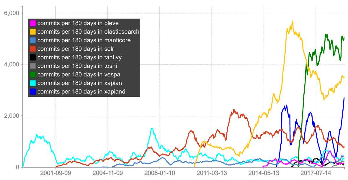
To visualize the size of these projects, here is the number git commits over time (compared to ES). One thing to note is that Lucene and Solr lives in the same git repository (and ES uses Lucene). Also, note that the first commit in the Vespa repository is a 2.5 MLOC behemoth diff that represents the squashed history up to that point (i.e. this codebase is literally decades old).
I also plotted the number of commits pushed to each project per 180 day window (this says nothing about the quality or size of the commits ofc). It shows that Vespa has a higher commit rate than ES right now:
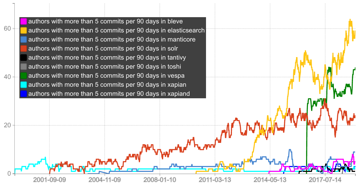
This final plot shows the number of git authors with 5 or more commits per 90 days (I use this as a proxy metric for counting the number of “full time developers” working on a project). For example, the Xapiand project have essentially 3 developers working on it:
How Elasticsearch is licensed
In ES 6.2 and earlier, the Elasticsearch Github repository contained only Elasticsearch and Elasticsearch was and is open source. On top of that, there has always been a set of commercial plugins available as a separate download called X-Pack. Even, critically important functionality like authentication and TLS was part of X-Pack, which also contained functionality for alerting, reporting and some machine learning features. For Elasticsearch 6.3, Elastic decided to add all the X-Pack code into the main Elasticsearch git repository but the new code was still not published under an open source license like the rest of Elasticsearch. Shay Banon described the rationale for that change here.
There are various projects that tries to offer open source replacements for the X-Pack plugins. For example, SearchGuard is an open source authentication plugin for Elasticsearch, even though they eventually launched a paid version of their open source plugin. There is an overview of various X-Pack alternatives available here.
AWS offers a hosted Elasticsearch service which runs a slightly modified version of Elasticsearch (which is API compatible with the open source version of ES for the most common API calls). This service offers authentication for example, but it does not have X-Pack installed. This service competes with the hosted cloud service that Elastic themselves maintain where you get ES instances with X-Pack preinstalled.
In March 2019, AWS launched Open Distro for Elasticsearch which is essentially a set of open source ES plugins that AWS uses to provide security, alerting, SQL support and performance analysis tools.
Example of what Elasticsearch offers: Search
Elasticsearch offers synonymization, handling of typos, match highlighting, auto completion and it can compute a relevance score for each search result indicating how well that particular item matched the search query. In particular:
-
Synonymization allows you to configure your indexing so that a document that mentions a “courageous knight” is returned whenever a user searches for “brave knight” and so on, based on custom or predefined lists of synonyms.
-
Typo handling ensures that a document that mentions something “outrageous” is found when a user searches for “outragous” (or vice versa). ES also comes with a “Phrase Suggester” that can be used to implement “Did you mean XYZ” suggestions to the end user.
-
Match highlighting gives you a machine readable map of which particular words matched which search term (so that you can make them bold in the search results or similar).
-
Auto complete can be implemented using ES in-memory “completion suggesters”.
-
Relevance scoring means that documents that match the search query very well will be given a higher score and will be returned up top among the search results.
It’s not a good idea to rank documents based only on the number of search terms
they contain, because suppose you had a database of recipes and two of them were
titled How to make the best pasta ever and Tasty Fudge. If a user
searches for how to make the tastiest fudge ever and you only ranked
results based on the number of search terms that matched, then the pasta recipe
would get the highest ranking because 5 words/terms are matching, whereas with
the fudge recipe there is only one match (or two if you have enabled stemming so
that tasty/tastiest count as a match). If the database has many recipies with
titles that begin with How to make then matches for the words how,
to and make are not going to be very useful for understanding which
document(s) the user is really looking for.
The problem is that matches for common words like “the” and “to” should not increase document ranking as much as a match for the less common word “fudge”. This idea is formalized in an algorithm called TF/IDF which stands for Term Frequency / Inverse Document Frequency. This algorithm was the default algorithm for relevance ranking in ES for many years. In practice though, extremely common words like “the” was often not even indexed in the first place (such words are referred to as stopwords) but the general idea holds; that matches for less common terms cause higher relevance scores compared to hits for words that are more common in the overall index. Other than term frequence and inverse document frequency, Elasticsearch also computes something called the “field-length norm” which means that if two documents both have a single match, but one of the documents have the match in a shorter field, then that document gets slightly higher relevance score. You can also customize relevance scores heavily, for example you might want to let a “product rating” field weigh into the ranking.
The current version of Elasticsearch uses another algorithm called Okapi BM25 for computing relevance scores. This algorithm is quite similar to TF/IDF but handles stop words more gracefully.
Example of what Elasticsearch offers: Cardinality Estimation
When a SQL database executes a query like SELECT COUNT(DISTINCT(type)) FROM
products it will insert all .type values into a hash set and then count
the number of elements in the end. If the dataset had N values and M
unique values, then this requires O(M) memory and takes O(N) time
(since each hash set insert takes O(1) amortized). For high cardinality
sets, M might exhaust available RAM so that the database needs to sort it on
disk there which is very slow. Also, if you split the data into two parts and
determine the number of unique .type values in each part, that information
cannot be combined to deduce the number of unique .type values in the entire
dataset. If the set of unique values is so large that it needs to span across a
large cluster of machines, then the above algorithm is simply impracticable.
This problem is called the count-distinct
problem.
There are radically more efficient algorithms available, given that you are willing to settle for approximately correct counts. For example, you could hash all your items into integers and set them in a bitset (this has the same time complexity but it has orders of magnitude better space complexity but of course each hash collision would cause the final count to be slightly off); this is called “linear counting”. An even better solution was published in 1984, namely the Flajolet–Martin algorithm. Eventually that work was refined into “LogLog Counting”, which in turn evolved into HyperLogLog (HLL, the most commonly used algorithm for this problem today) which was first published in 2007 by Philippe Flajolet et al. In general, HLL is a cornerstone of “big data” and variants of this algorithm is used in Redis, Spark, Redshift, BigQuery etc. The HLL commands in Redis are prefixed with “PF” in honor of Philippe Flajolet.
If you count the number of distinct words in Shakespeare’s works using a hash set, linear counting and HLL you get these results:
| Counting Algorithm | Bytes Used | Count | Error |
|---|---|---|---|
| HashSet | 10447016 | 67801 | 0% |
| Linear Counting | 3384 | 67080 | 1% |
| HyperLogLog (HLL) | 512 | 70002 | 3% |
The cardinality aggregation feature in Elasticsearch uses a slightly improved HLL variant called HyperLogLog++, and this makes it possible to count the number of distinct elements in a field on a per shard basis and then use the results of those computations to provide an approximate total. This algorithm is explained more in-depth by Adrien Grand (ES/Lucene committer) in this video.
Nodes, Shards, Indices and Routing
An Elasticsearch cluster consists of a set of nodes (typically a node is a
single machine running ES). Elasticsearch stores documents (essentially blobs of
JSON) into indices; an ES index is conceptually similar to SQL table. Each
document is marked with a built-in field called “_id” which uniquely identifies
that document. An ES cluster can have multiple indices, for example one for
“products” and one for “customers”. Each index is typically partitioned into
primary shards so that each document is stored in exactly one primary shard. For
example, you can load a document with ID UMNkYH from the products
index using:
$ curl -s 'es-hostname:9200/products/_search?q=_id:UMNkYH'
When ES receives a “find by document id” request like this, it will hash the document ID to determine which primary shard the document is stored in (this process is called routing). Similarly, when a set of new documents are inserted into the index, the uniformity of the hash function ensures that they are added evenly across all shards. The number of shards is set when the index is created and can not be changed, unless you create a new index and reinsert all your data into it (which often ends up being a quite expensive operation). When ES receives a regular search request like “find all products with a price below 100” or “find all documents that contain the words foo and bar”, it does not know which shards contain the requested documents so it will instead broadcast the query to all shards and then merge the results from each shard.
How to execute basic queries
There are two formats that can be used when sending queries to ES. The curl
command in the previous section runs a URI
search
and passes the search criteria via the q= parameter. The other format is
request body
search
where the search criteria is passed as JSON in the request body instead. If you
rewrite the “find by id” query from above as a request body query you get:
$ curl -s 'es-hostname:9200/products/_search' -H "application/json" \
       --data-raw '{"query":{"term":{"_id":"UMNkYH"}}}'
ES returns JSON and you can get it pretty-printed by adding pretty as a URL param to the request:
$ curl -s 'es-hostname:9200/products/_search?q=price:42&pretty'
$ curl -s 'es-hostname:9200/products/_search?pretty' -H "application/json" \
       --data-raw '{"query":{"term":{"_id":"UMNkYH"}}}'
Another (better) way to pretty print the JSON is to pipe it to jq or fx.
The syntax used within the q= is very similar to the Lucene syntax you
enter in Kibana. Although, you have to keep URL escaping in mind so replace
space with + etc. For example, if you want to find all products with
category set to “camera” and a price of 1999, use:
$ curl -s 'es-hostname:9200/products/_search?q=price:1999+AND+category:camera' | \
    jq -C . | less -RSFX
When you need to query datetime fields with this syntax ES offers some basic
“date math” support that you can use within square brackets. However, note that
curl processes square brackets as shell globbing unless you pass the -g
parameter to curl. So if you need to find all products postings with category
“camera” that was modified in the last 3 hours, use:
$ curl -s -g 'es-hostname:9200/products/_search?q=lastmodified:[now-3h+TO+now]' | \
    jq -r .hits.total
In ES versions before 5.x, a lot of people installed a plugin called
kopf. This plugin allowed you
to get an overview of nodes, shards, indices and it also had a “rest” tab where
you could submit JSON queries. If the kopf plugin is installed, you can open it
by navigating to es-hostname:9200/_plugin/kopf. In ES 5.x and later you
can use cerebo which is essentially kopf
but as a standalone program (written by the same author).
Another really nice way to submit JSON queries is via the “devtools console” in Kibana.
Examples of a few other ES API calls
# Show cluster name, health and node/shard count
$ curl -s 'es-hostname:9200/_cluster/health' | \
    jq -r '{ cluster_name, status, number_of_nodes, active_primary_shards }'

# List available indices
$ curl -s 'es-hostname:9200/_cat/indices'

# List available indices, with column captions
$ curl -s 'es-hostname:9200/_cat/indices?v'

# List available indices, storage sizes in bytes instead of human readable units
$ curl -s 'es-hostname:9200/_cat/indices?v&bytes=b'

# List nodes with current CPU/mem usage
$ curl -s 'es-hostname:9200/_cat/nodes?v'
Replicas and cluster health
Each primary shard is stored on a single node, but each node can manage several shards. If more nodes are added, the ES cluster automatically rebalances itself by moving a few shards over to the newly added nodes. Each index also has a replica count defined which ensures that for each primary shard there is also N identical “replica shards” that are kept up to date at all times. For example, if you set the replica count to 1, ES writes all data to both the primary shard and the replica and it constantly works to ensure that the replica lives on a different node from the primary. If a machine malfunctions ES can promote a replica to primary or spawn a new replica. All incoming writes are executed on both the primary and the replica shard, but reads can be served directly from a replica shard so other than failover they also improve read performance.
If ES is unable to maintain the configured replica count, the index health status changes from green to yellow (and to red if data is lost). This also means that the overall cluster health status changes. You can see the cluster health status using the _cluster API call from the previous section. Tools like kopf/cerebro make is quite clear that the cluster is unhealthy, for example cerebro renders a the line underneath the main menu using the cluster health status color. When the cluster switches from unhealthy to healthy this line goes from yellow to green. When it’s yellow you typically also see some error message saying that you have for example “15 unassigned shards”. The default replica count is 1 so whenever you add data to ES on localhost for development purposes, the cluster health immediately becomes unhealthy/yellow since the localhost “cluster” only has a single node so ES cannot store the replica on a different node from the primary. You can fix this by selecting the dropdown menu on the index which has “unassigned shards”, then select “index settings” and set the replica count to 0 (NOTE: only do this for localhost dev instances where you don’t want replication).
Rollover Indices
When you store immutable chronological data like logs (and also recorded
metrics), it’s quite common to write the data into an index where the name
contains a timestamp, for example logstash writes to logstash-yyyy.mm.dd
by default. If you want to delete the oldest data periodically you can do this
by deleting an entire index at once (which is much faster and more resource
efficient than trying to delete documents inside a single index). When you do
this, you would typically define an index
template
in ES that specifies the settings that should be used whenever a new
logstash-* index is created (i.e. the number of shards/replicas as well as
the field mappings and so on).
People have been using setups like that for years, but there are some drawbacks with it; for example since all write operations target the active index (and for use cases like this often a majority of the read queries target the active index as well) you often want more nodes backing the active index compared to older indices. Also, it’s quite common that not “all days are the same” (e.g. you might be process log data for a stock exchange that happens to be closed during weekends). To mitigate these issues you can use the rollover API instead, which allows you to specify conditions for new index creation on a more granular basis and since the data is immutable you can automatically force merge older indices and move them off hot nodes (assuming the cluster is setup with hot warm architecture).
Memory for ES
Just like other large JVM applications, ES is sensitive to the Java heap limit
for compressed ordinary object
pointers
(oops). If you give a Java process 31gb or less memory it can use 32-bit
pointers and multiply them to by 8 to find the real address. If you give it
33gb, the JVM will start in 64-bit pointer mode instead and since ~20% of any
Java heap is object pointers, you will have less actual memory availble compared
to running with the 31gb limit. Running with limited Java heap is not a problem
since you can use more nodes instead. There is also an even more efficient mode
called “zero based compressed oops” and to use this mode you need ~26GB or less
Java heap. Also, as with other Java applications; resizing the heap at runtime
can be quite slow so it’s a good idea to run with identical min/max values, e.g.
-Xms31g -Xmx31g. By default, ES starts with 1GB heap which is pretty much
always wrong for production clusters, you can configure your JVM heap options in
the file config/jvm.options. You can also configure which JVM GC to use in
this file, notably the Java 8 G1GC has less stop-the-world GC pauses compared to
the default CMS collector.
Because Lucene uses quite a lot of disk-backed data structures, so it’s
important to leave memory (ideally at least 50% of physical RAM) for operating
system file caches. If you use a smaller Java heap for ES you get shorter GC
pauses and more memory for Lucene’s file system caches. If you won’t be
aggregating on analyzed string fields you can make the ES Java heap even smaller
than 50%. You should also disable
swapping,
either completely using sudo swapoff -a, and/or by setting
bootstrap.memory_lock: true in elasticsearch.yml. Even if you
allocate plenty of memory for file system caches, it’s often a good idea to use
fast SSD disks (and if you do, double check cat
/sys/block/{DEVICE-NAME}/queue/scheduler so you’re not accidentally using
cfq which is not suitable for SSDs). You can setup RAID 0 if you want (but
skip other RAID variants since failover is handled by replicas).
The Inverted Index vs Doc Values
The main data structure backing full text analyzed fields in ES is an inverted index that maps terms to a set of postings (document IDs of documents containing that term). For example:
    "berry"    -> { freq: 4, postings: [2, 42, 55, 88]            }
    "fish"     -> { freq: 6, postings: [1, 42, 55, 88, 91, 92]    }
    "pasta"    -> { freq: 5, postings: [4, 5, 55, 67, 111]        }
    "red"      -> { freq: 3, postings: [6, 7, 99]                 }
    "zucchini" -> { freq: 1, postings: [121]                      }
Because the terms in the left column are sorted alphabetically, it’s possible to find search terms quickly in that list and hence also the associated document IDs. This is a good data structure for answering queries like “find documents matching ‘red berries’” because ES can just normalize each search word using the configured analysis algorithm (so that “berries” becomes “berry” for example), and then lookup the matching documents. ES tracks various other information like “term frequency” (number of documents in the index that contains the relevant term) and “which character offset the term appeared at inside the field” etc. Also on a lower level, Lucene considers the same string in different fields to be different terms (i.e. a Lucene term is essentially tuple of (FIELD_NAME, SOME_WORD)).
For use cases where you instead want to sort, aggregate or use field values from
scripts, the inverted index is not a suitable data structure, but ES can also
store the data in another way, namely as doc
values.
They are essentially an inverted inverted index because given a field name and a
document ID you can use the doc values data structure to efficiently retrieve
the value of that field in the given document. Doc values are supported for all
fields that are not analyzed strings (i.e. all field data types except “text”),
and they are enabled by default whenever they are supported. If you are
absolutely sure that you will never need to aggregate or sort based on a field
you can set doc_values: false in the mapping and save a small amount of
disk space and gain some indexing speed. Note that doc values are stored in a
disk based data structures and read via the file system cache (just like the
Lucene indices) so they don’t bloat the ES Java heap.
For example, imagine we have an ES index with recipes and each recipe has fields for “title”, “cooking_instructions”, “minutes_required” as well as a “recipe_type” field that indicates whether the recipe is a “entrée”, “main course” or “dessert”. It makes sense to store “title” and “cooking_instructions” as text fields (analyzed) so we can do full text search over them, but we will store the “minutes_required” field as an integer so that we can sort the recipes by how long they will take to prepare. For “recipe_type” we will use the datatype “keyword” which is a non-analyzed string type, ensuring that we’ll have doc values available so we can use this field for aggregation (e.g. calculate the number of recipes of each “recipe_type”).
However, we might also want to generate a list of recipes sorted by their
“title” but since “title” is a text field we cannot use it for sorting. You
could overcome this by indexing the recipe title into two different fields, one
with datatype “text” and another with datatype “keyword”) but this would cause
some storage overhead in the _source metafield. A better solution is to
declare a single multifield mapping that will store the data in both formats at
once, so instead of "title": { "type": "text" }, you would use a mapping
like:
    "title": {
        "type": "text",
        "fields": {
            "keyword": {
                "type": "keyword"
            }
        }
    },
Multifields like the above are also used by logstash by default which is why you often see both “foobar” and “foobar.raw” when you query data in Kibana.
FieldData
As outlined in the previous section, you should always use doc values for all fields that you will use for aggregation and sorting. Strictly speaking though, it is possible to execute an aggregation query for a field that contains analyzed text, but often it is not a good idea to do this because A) it can lead to memory related performance problems, and B) the result of such aggregation is quite often not what the caller expected.
The memory issues happens because analyzed text fields are stored as an inverted tree (see earlier section) but aggregation would need a data structure similar to doc values to run efficiently. So, when ES is asked to aggregate over a field that contains analyzed text, it will (at query time!) invert the inverted tree and then also cache the inverted inverted tree permanently on the JVM heap. This in-memory data structure is called fielddata. Unlike memory used by Lucene via the file cache, this fielddata cannot be reclaimed by the OS if the machine runs low on memory.
It’s sufficient for a single “one off” aggregation on analyzed text to generate
and permanently keep this fielddata in memory, after which Lucene will have less
memory to work with and every single GC will take longer to process. Logstash
tends to use multifields so you get both “component” and “component.raw” (where
the latter is using doc values) and a single innocent pie chart aggregation on
“component” could, in theory at least, permanently impair cluster performance.
In reality, this particular case is blocked since the analyzed text field
“component” would likely be marked with "fielddata" : { "format" :
"disabled"} which means that you’d get an error in Kibana if you tried to
generate such a pie chart of death. The right way is to aggregate based on
“component.raw” instead.
You can see how much fielddata you have allocated for each node, by running:
$ curl -s 'es-hostname:9200/_cat/fielddata?v&fields=*'
It is possibe to clear the fielddata cache using curl -s
'localhost:9200/_cache/clear?fielddata=true' but this will of course cause
performance issues if your application relies on this data.
When it comes to B) above (why aggregation on analyzed text often doesn’t produce the desired result anyway), consider this this example:
curl -s -X PUT localhost:9200/bad_recipes
curl -s -X PUT -H "Content-Type: application/json" \
     localhost:9200/bad_recipes/_mapping/_doc --data-raw '
{
  "properties": {
    "title": {
        "type": "text",
        "fields": {
            "keyword": {
                "type": "keyword"
            }
        }
    },
    "recipe_type": {
      "type": "text",
      "fielddata": true
    }
  }
}
' | jq .
curl -s -X POST -H "Content-Type: application/json" \
     'localhost:9200/bad_recipes/_doc' \
     --data-raw '{"title": "first title", "recipe_type": "main course" }' | jq
curl -s -X POST -H "Content-Type: application/json" \
     'localhost:9200/bad_recipes/_doc' \
     --data-raw '{"title": "second title", "recipe_type": "dessert" }' | jq
curl -s -X POST -H "Content-Type: application/json" \
     'localhost:9200/bad_recipes/_doc' \
     --data-raw '{"title": "third title", "recipe_type": "weird" }' | jq
curl -s -X POST -H "Content-Type: application/json" \
     'localhost:9200/bad_recipes/_doc?refresh=wait_for' \
     --data-raw '{"title": "fourth title", "recipe_type": "weird" }' | jq
curl -s -H "Content-Type: application/json" \
     localhost:9200/bad_recipes/_search \
     --data-raw '{"aggs":{"my_agg_name":{"terms":{"field":"recipe_type"}}}}' | jq
The final aggregation outputs the following buckets:
      ...
      "buckets": [
        {
          "key": "weird",
          "doc_count": 2
        },
        {
          "key": "course",
          "doc_count": 1
        },
        {
          "key": "dessert",
          "doc_count": 1
        },
        {
          "key": "main",
          "doc_count": 1
        }
      ],
      ...
That is, because the field contains analyzed text the value “main course” was treated as the field having two values “main” and “course” and the aggregation was computed accordingly (i.e. the counts are “wrong”).
Because it is easy to shoot yourself in the foot with fielddata, it has been
disabled by default in recent ES versions, which is why the above example has
"fielddata": true in the mapping. In older versions of ES (e.g. 2.x)
fielddata was enabled by default, and in ES 1.x doc values were also disabled by
default, making the pit of success even smaller.
There are use cases where aggregation on analyzed text does give the correct output; for example if you wanted to make a tag cloud (word cloud) visualization so that words that appeared more often was rendered with a bigger font size etc and you didn’t want to do this for the entire index but rather for a subset of documents. Another such use case is significant terms aggregation.
Refresh
When you write data into ES you cannot find it using a search until after the next “refresh”. By default the refresh interval in ES is 1s, but this can be tweaked to a higher value to give ES more room to optimize throughput. You can see the current refresh interval for a given index using:
$ curl -s es-hostname:9200/indexName/_settings \
      | jq -r 'to_entries | .[0].value.settings.index.refresh_interval // "1s"'
When you write data to ES with curl you can pass ?refresh=wait_for if you
want it to block until the data is visible to searches.
More About Elasticsearch
- Designing the Perfect Elasticsearch Cluster: the (almost) Definitive Guide by Fred de Villamil
- Running Elasticsearch for Fun and Profit
- awesome-elasticsearch repo on GitHub
1: https://github.com/kimchy/compass
2: Elasticsearch blog: Welcome Jordan & Logstash
3: Marc Gravell, who works for Stackoverflow, described the reasons why they moved away from MSSQL full text search to Elasticsearch in this comment (from 2013). They periodically post details of their setup, including how they use Elasticsearch.
4: For example, MySQL has support for full text search via ```MATCH() ... AGAINST``` but as soon as you combine such a search with a regular SQL condition performance suffers heavily.